Axis Bank Share Price Analysis: RSI (14) at 40.8 and Close 15.0% Below Its 52-Week High on 27 October 2026

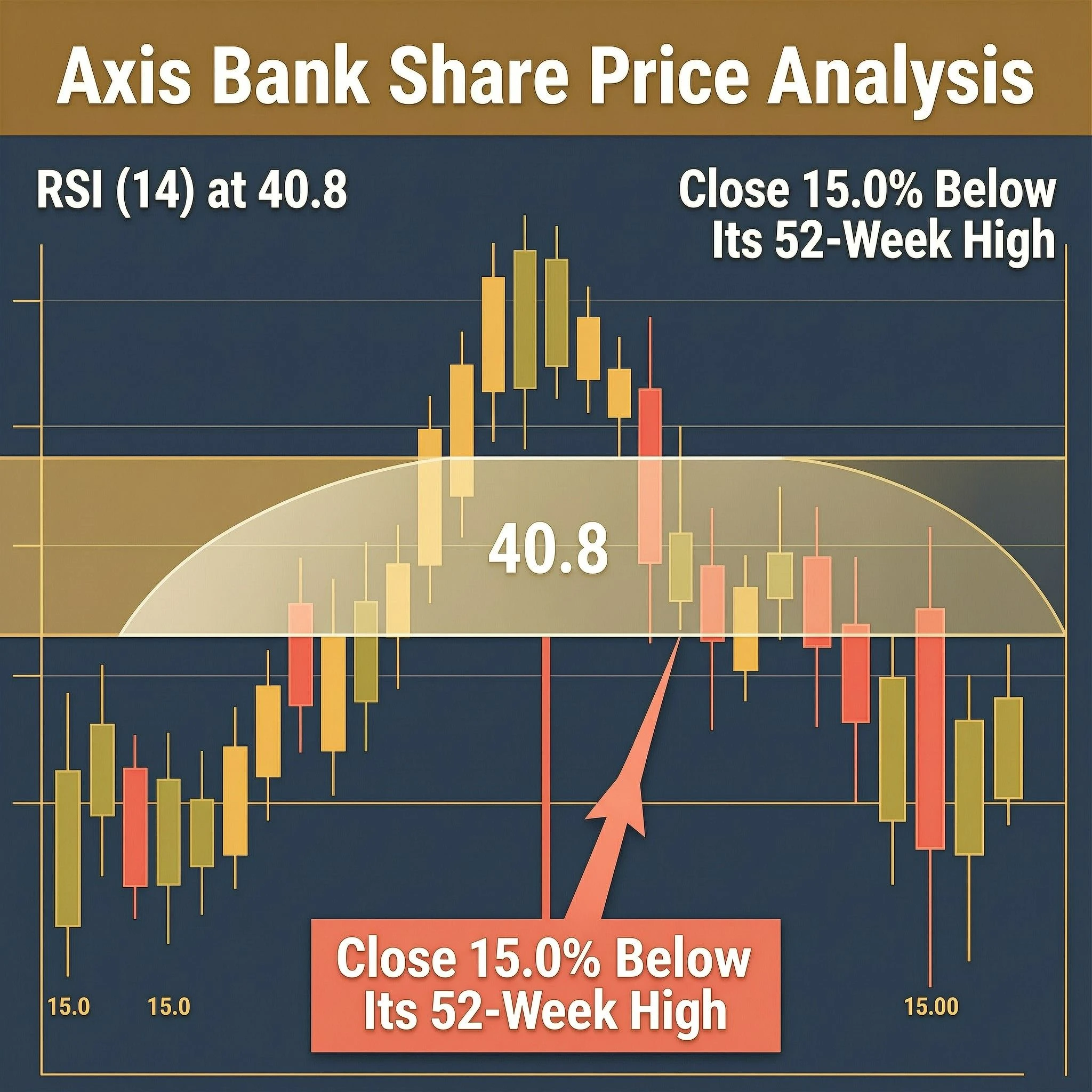
Axis Bank Ltd. closed at ₹1,205.70 on 27 October 2026, a decline of 1.17% from the previous close of ₹1,220.00, and the session's trading range of ₹1,205.70 to ₹1,229.20 placed the stock near the bottom of its daily band.

Volume of 70.2 L came in at 0.9× the 20-day average of 76.9 L, a reading that suggests participation was lighter than usual rather than heavier. The close sits 15.0% below the 52-week high of ₹1,418.30 recorded on 3 February 2026 and 4.8% above the 52-week low of ₹1,150.30 set on 2 April 2026, framing a stock that has spent most of the year in a wide but well-defined corridor.

What follows is a structured reading of the technical record as it stood at the NSE end-of-day print on that date. Each section takes one indicator or dataset, explains in plain language what it measures, and then reports the verified figures exactly as computed from stored prices.

The note covers the price snapshot, returns across six horizons, trend and risk context, and then the five indicator families plotted on the charts: Bollinger Bands, RSI, the simple moving average, the Z-Score and the linear regression line. Corporate actions and the last five sessions close out the factual record.

No cause is assigned to any move, because the data brief does not supply one. The purpose here is descriptive and educational: to show how a set of standard technical readings can be assembled into a coherent picture of where a large-cap private bank stock stood on a single trading day, and to explain the arithmetic behind each measure so that readers can interpret similar figures on their own.

TL;DR Axis Bank Ltd. closed at ₹1,205.70 on 27 October 2026, down 1.17% on the day, 15.0% below its 52-week high and 2.9% below its 50-day simple average, with RSI (14) at 40.77 and a Z-Score (20) of -1.23.

Snapshot

The snapshot fixes the single most important reference point in any technical note: the closing price and the context immediately around it. Axis Bank ended the session at ₹1,205.70, having traded between ₹1,205.70 and ₹1,229.20 during the day.

The day-over-day change was -1.17%, measured against the prior close of ₹1,220.00, and the closing print landed at the very bottom of the intraday range.

Volume is the second anchor. Turnover of 70.2 L compared with a 20-day average of 76.9 L, a ratio of 0.9×, which means the session traded slightly below its recent typical participation.

Volume surge against the 20-day average is a common way to judge whether a price move carried conviction; here the ratio points to a quieter-than-average session rather than an outsized one.

The 52-week envelope gives the longer frame. The high of ₹1,418.30 was set on 3 February 2026, and the close is 15.0% below it. The low of ₹1,150.30 came on 2 April 2026, and the close is 4.8% above it.

The stock therefore sits in the lower portion of a range that has been roughly 23% wide from trough to peak over the year.

Price change over time

Returns across several horizons show whether a single session's move is an isolated event or part of a broader pattern. Axis Bank's record over the six measured windows is uniformly negative except at the longest horizon, and the magnitudes are modest at every step.

The five-day figure of -2.5% is the largest short-term decline, while the one-month and three-month readings of -1.4% and -1.5% are close to flat.

The medium-term windows deepen the picture. Over six months the stock returned -6.5%, and over one year -3.9%, both consistent with a stock that has drifted lower without a sharp break.

The three-year figure of +20.2% is the only positive entry, and it captures a much longer cycle than the technical indicators in later sections, which are all computed over windows of 20 days or less.

• 5 days: -2.5%
• 1 month: -1.4%
• 3 months: -1.5%
• 6 months: -6.5%
• 1 year: -3.9%
• 3 years: +20.2%

Read together, the sequence describes a stock that has given back ground gradually over the past year while still holding a positive cumulative return over three years. The absence of a large one-year loss alongside a 15.0% gap to the 52-week high indicates that the peak was reached early in the window and the subsequent path was a slow decline rather than a single collapse.

Trend and risk context

Moving averages and risk statistics place the closing price inside a broader structure. The close is 2.9% below its 50-day simple average of ₹1,242.25 and 6.1% below its 200-day simple average of ₹1,284.04.

A simple moving average is the plain mean of the last N closes, and it smooths day-to-day noise to reveal the prevailing direction. The 50-day average sitting below the 200-day average is a configuration that describes a medium-term trend weaker than the long-term one.

Risk is measured here in three ways. The deepest fall from a closing high within the last year was 17.2%, which is the maximum drawdown over that window. Annualised volatility of daily returns over the last 60 sessions is 23.3%, a figure that scales the standard deviation of daily moves to a yearly basis.

The 14-day average true range is 2.3% of the close, expressing the typical daily trading range as a share of price.

The extremes of the last three months add texture. The best single day was +3.46% on 3 August 2026, and the worst was -4.56% on 24 September 2026. A spread of roughly eight percentage points between the best and worst sessions, against an annualised volatility of 23.3%, describes a stock with meaningful but not extreme day-to-day swings.

• 50-day simple average: ₹1,242.25 (close 2.9% below)
• 200-day simple average: ₹1,284.04 (close 6.1% below)
• Maximum drawdown, last year: 17.2%
• Annualised volatility, 60 sessions: 23.3%
• 14-day average true range: 2.3% of the close
• Best day, last three months: +3.46% on 3 Aug 2026
• Worst day, last three months: -4.56% on 24 Sep 2026

Chart: Bollinger (20, 2)

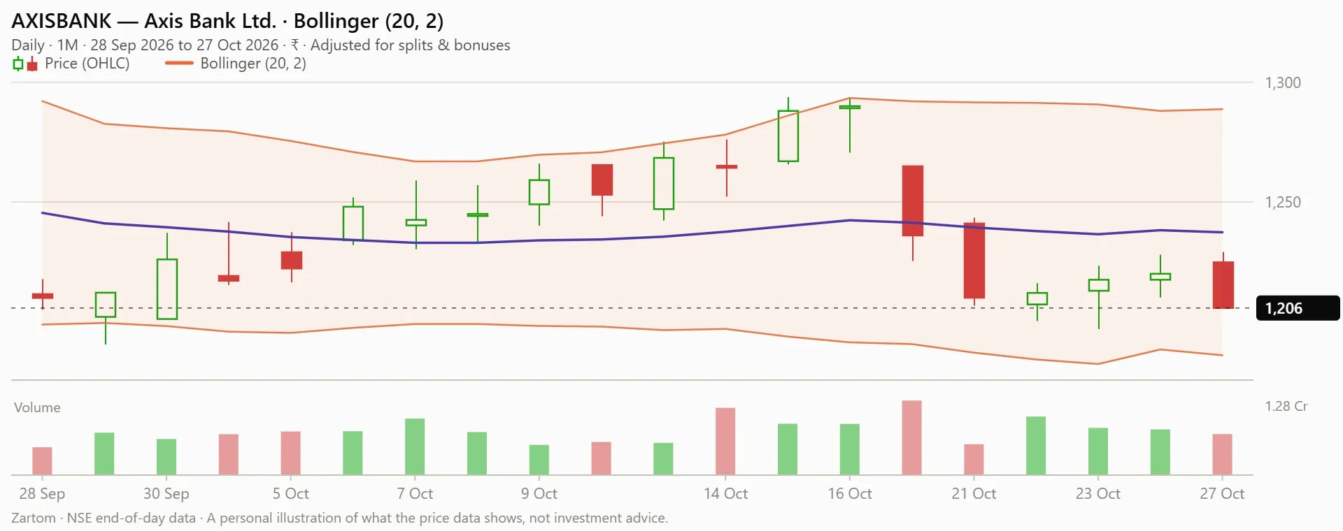
The Bollinger chart plots the daily closing price with volume at the base, overlaid with a 20-period average and two standard-deviation bands either side of it. It is the first of five indicator charts in this note, and each follows the same layout so that price, volume and the indicator can be read together on a single canvas.

Bollinger (20, 2): what it shows

Bollinger Bands are an average with bands K standard deviations either side of it, and the bands widen when volatility rises. The settings here are a 20-period base and 2 standard deviations.

The upper band stands at 1,289, the middle at 1,237 and the lower at 1,186, so the close of 1,206 sits 6.4% below the upper band, 2.6% below the middle and 1.7% above the lower.

Each band's position within its own one-year history is informative. The upper band is at the 27th percentile of its yearly range of 1,214 to 1,457, the middle at the 15th percentile of 1,170 to 1,362, and the lower at the 18th percentile of 1,118 to 1,320.

All three sit in the lower part of their annual distributions, and the middle line has fallen 0.9% over the last 20 sessions.

• Upper band: 1,289, changed by −3.25 over 5 sessions and −3.86 over 20
• Middle band: 1,237, changed by −3.98 over 5 sessions and −10.85 over 20
• Lower band: 1,186, changed by −4.71 over 5 sessions and −17.83 over 20
• Band width: 8.3% of the midpoint, wider than 52% of last year's readings
• %B: 0.19, placing the close in the lower fifth of the bands

The close last crossed below the upper band on 16 October 2026 and below the middle on 19 October 2026, having crossed the upper 18 times and the middle 23 times in the last year.

It last crossed above the lower band on 25 September 2026, with 12 such crossings over the year. The bands are 8.3% wide relative to their midpoint, a width wider than 52% of the past year's readings.

The calculation behind this indicator, with a worked example from this stock's own prices, is shown below.

Learn: how the Bollinger (20, 2) is calculated

Bollinger Bands put a band above and below a moving average. The band is as wide as the recent day-to-day variation of the price, so it widens when prices swing more and narrows when they are quiet.

The mathematics

The middle line is the ##N##-day simple average, and ##\sigma_t## is the standard deviation of the same ##N## closes:

###M_t = \frac{1}{N}\sum_{i=0}^{N-1} C_{t-i}, \qquad \sigma_t = \sqrt{\frac{1}{N}\sum_{i=0}^{N-1}\left(C_{t-i} - M_t\right)^2}###

With a multiplier ##k## (usually 2) the bands are

###U_t = M_t + k\,\sigma_t, \qquad L_t = M_t - k\,\sigma_t###

Two readings derived from the bands are the position within them and their relative width:

###\%B_t = \frac{C_t - L_t}{U_t - L_t}, \qquad \text{width}_t = \frac{U_t - L_t}{M_t}###

Worked example with this instrument's latest numbers

Over the last 20 closes the average is ₹1,237.36 and the standard deviation is ₹25.70, so the upper band is ₹1,288.75 and the lower band ₹1,185.96. The latest close of ₹1,205.70 sits 19% of the way from the lower to the upper band.

###U = 1237.36 + 2 \times 25.70 = 1288.75, \qquad L = 1237.36 - 2 \times 25.70 = 1185.96###

These figures are computed from the same prices as the chart above, so the result matches the indicator's latest reading.

In Python (pandas)

import pandas as pd

def bollinger(close: pd.Series, n: int = 20, k: float = 2.0) -> pd.DataFrame:
    """Bollinger Bands with the population standard deviation (ddof=0)."""
    middle = close.rolling(n).mean()
    spread = close.rolling(n).std(ddof=0)
    return pd.DataFrame({"lower": middle - k * spread, "middle": middle, "upper": middle + k * spread})

Going deeper

• This app uses the population standard deviation (divide by N). Some software divides by N−1; the bands differ slightly (by a factor of about 1.026 for N = 20).
• The popular statement that about 95% of closes fall inside two-standard-deviation bands is true only for normally distributed values. Daily price changes have fatter tails, so more closes than that land outside in practice.
• The standard deviation is taken of the prices, not of returns, so a steady trend widens the bands even without large daily moves.
• Band width is often compared with its own history (percentile over a year) to say whether the stock is unusually quiet or active.

Relation between the width and the spread:

###\text{width}_t = \frac{2k\,\sigma_t}{M_t}###

A further Python version

def bollinger_with_stats(close, n=20, k=2.0):
    mid = close.rolling(n).mean()
    sd = close.rolling(n).std(ddof=0)
    upper, lower = mid + k * sd, mid - k * sd
    pct_b = (close - lower) / (upper - lower)
    width = (upper - lower) / mid
    width_rank = width.rolling(252).apply(lambda w: (w <= w.iloc[-1]).mean() * 100, raw=False)
    return pd.DataFrame({"lower": lower, "middle": mid, "upper": upper, "pct_b": pct_b, "width": width, "width_percentile": width_rank})

Try it yourself

For these closes and N = 5, k = 2, give the middle line and the population standard deviation on the last day.

data = [44,46,45,47,49]

Answer: 46.2, 1.72.

Chart: RSI (14)

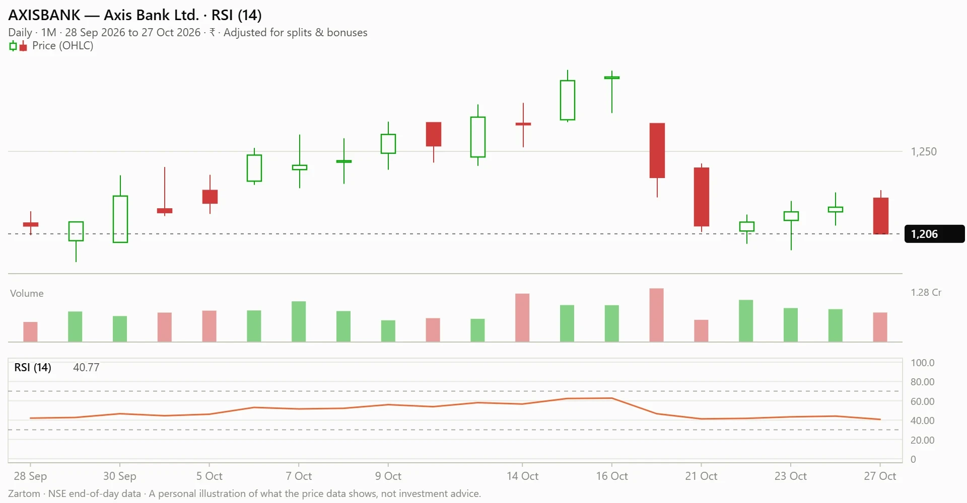
The RSI chart shows the daily price with volume at the base and the 14-period relative strength index plotted beneath it. The indicator compresses recent gains and losses into a single line on a 0–100 scale, which makes it easy to see how the balance of up days and down days has shifted over the recent past.

RSI (14): what it shows

The relative strength index compares recent gains with recent losses on a 0–100 scale, and readings above 70 are often described as stretched while those below 30 are described as depressed. The 14-day reading stands at 40.77, which places it between 30 and 50, in the lower half of the neutral range.

Over the last year the line ranged from 27.68 to 73.49 with a median of 52.18, so today's value sits at the 16th percentile of that distribution.

The recent direction is downward. RSI changed by −5.91 over the last five sessions and −3.95 over the last 20. Of the last 252 readings, only 3 (1%) were above 70 and 2 (1%) were below 30, so the indicator has spent almost the entire year inside the neutral band.

The line last rose through 70 on 19 November 2025 and last fell through 30 on 23 July 2026.

The calculation behind this indicator, with a worked example from this stock's own prices, is shown below.

Learn: how the RSI (14) is calculated

The Relative Strength Index compares how much the price has gained on its up days with how much it has lost on its down days over the last N days (14 by default), and squeezes the answer onto a scale from 0 to 100.

The mathematics

Gains and losses of day ##t##:

###G_t = \max(C_t - C_{t-1},\,0), \qquad L_t = \max(C_{t-1} - C_t,\,0)###

Wilder's smoothing keeps a running average (after an initial simple average of the first ##N## values):

###\overline{G}_t = \frac{(N-1)\,\overline{G}_{t-1} + G_t}{N}, \qquad \overline{L}_t = \frac{(N-1)\,\overline{L}_{t-1} + L_t}{N}###

The relative strength and the index:

###RS_t = \frac{\overline{G}_t}{\overline{L}_t}, \qquad RSI_t = 100 - \frac{100}{1 + RS_t}###

Worked example with this instrument's latest numbers

The latest close changed by −14.30 rupees from the day before. After Wilder's smoothing over 14 days, the average gain is 5.463 and the average loss is 7.935 rupees per day, so the relative strength is 5.463 ÷ 7.935 = 0.688 and the index is 40.77.

###RS = \frac{5.463}{7.935} = 0.688, \qquad RSI = 100 - \frac{100}{1 + 0.688} = 40.77###

These figures are computed from the same prices as the chart above, so the result matches the indicator's latest reading.

In Python (pandas)

import pandas as pd

def rsi(close: pd.Series, n: int = 14) -> pd.Series:
    """Relative Strength Index with Wilder's smoothing."""
    change = close.diff()
    gain = change.clip(lower=0)
    loss = -change.clip(upper=0)
    avg_gain = gain.ewm(alpha=1 / n, adjust=False).mean()
    avg_loss = loss.ewm(alpha=1 / n, adjust=False).mean()
    rs = avg_gain / avg_loss
    return 100 - 100 / (1 + rs)

Going deeper

• Wilder's smoothing is an exponential average with weight 1/N instead of 2/(N+1), so it reacts more slowly than a standard EMA of the same length.
• If there are no losses in the window the average loss is zero: RS is infinite and RSI is 100 (and 50 if there were no gains either). Implementations need to handle the division.
• RSI is bounded between 0 and 100, but how close it gets depends on the stock: a steady uptrend can keep it between about 40 and 90 for months, which is why the 30 and 70 lines are conventions, not boundaries.
• Because of the smoothing, the value depends (slightly) on how far back the data starts; after a few dozen days the difference is negligible.

The same index can be written directly from the averages:

###RSI_t = 100 \cdot \frac{\overline{G}_t}{\overline{G}_t + \overline{L}_t}###

A further Python version

def rsi_exact(close, n=14):
    """RSI seeded with the simple average of the first n gains and losses (the version used in this article)."""
    gains, losses = [0.0], [0.0]
    for i in range(1, len(close)):
        d = close[i] - close[i - 1]
        gains.append(max(d, 0.0)); losses.append(max(-d, 0.0))
    out = [None] * len(close)
    avg_g = sum(gains[1:n + 1]) / n
    avg_l = sum(losses[1:n + 1]) / n
    def value(g, l):
        if l == 0:
            return 50.0 if g == 0 else 100.0
        return 100 - 100 / (1 + g / l)
    out[n] = value(avg_g, avg_l)
    for i in range(n + 1, len(close)):
        avg_g = (avg_g * (n - 1) + gains[i]) / n
        avg_l = (avg_l * (n - 1) + losses[i]) / n
        out[i] = value(avg_g, avg_l)
    return out

In JavaScript

function rsi(close, n) {
  const out = new Array(close.length).fill(null);
  let g = 0, l = 0;
  for (let i = 1; i <= n; i++) { const d = close[i] - close[i - 1]; g += Math.max(d, 0); l += Math.max(-d, 0); }
  g /= n; l /= n;
  const value = (a, b) => (b === 0 ? (a === 0 ? 50 : 100) : 100 - 100 / (1 + a / b));
  out[n] = value(g, l);
  for (let i = n + 1; i < close.length; i++) {
    const d = close[i] - close[i - 1];
    g = (g * (n - 1) + Math.max(d, 0)) / n;
    l = (l * (n - 1) + Math.max(-d, 0)) / n;
    out[i] = value(g, l);
  }
  return out;
}

Try it yourself

With N = 3, work out the RSI from day 4 on (the first average is the plain mean of the first three gains and three losses).

data = [44,46,45,47,49,48,50,52,51,53]

Answer: (blank), (blank), (blank), 80, 87.5, 68.29, 80.88, 88.02, 68.77, 81.14.

Chart: SMA (20)

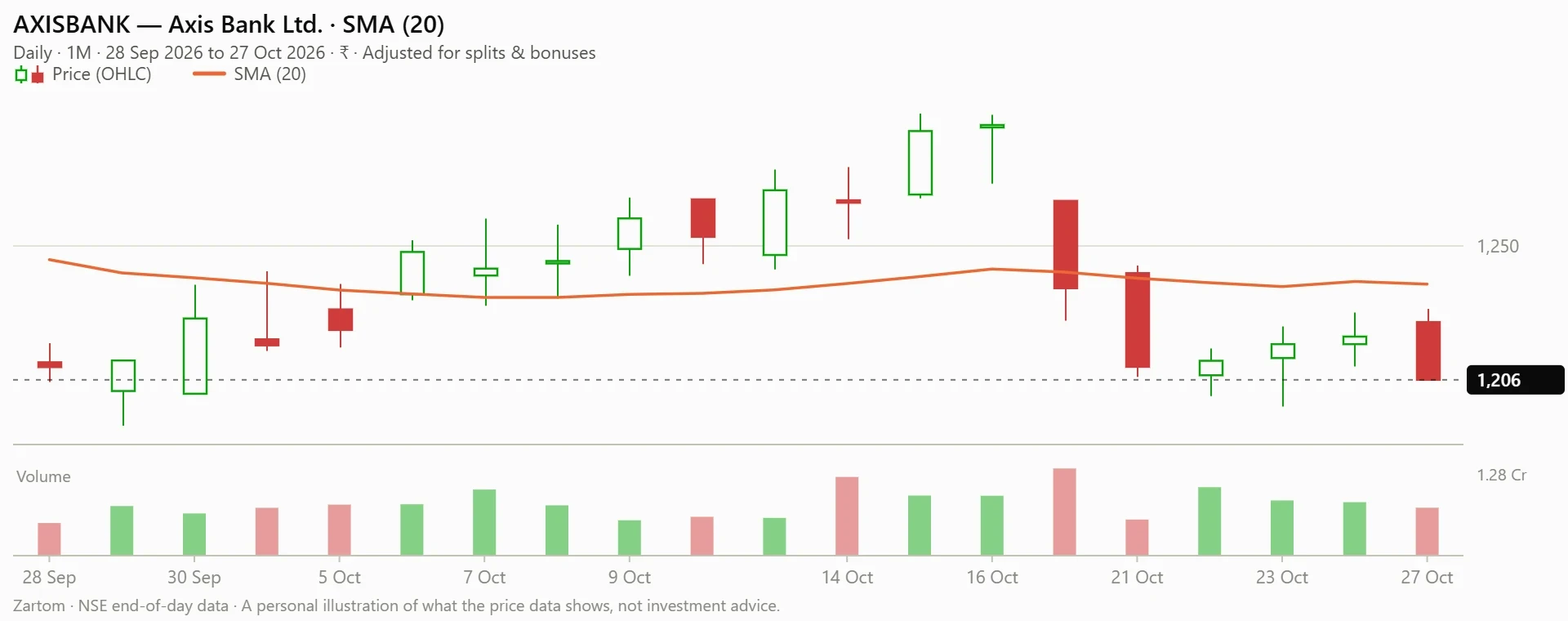
The SMA chart plots the daily price with volume at the base and a 20-period simple moving average drawn across it. Because the average is the plain mean of the last 20 closes, it responds slowly to new prices and gives a clean visual reference for whether recent trading has been above or below its own recent norm.

SMA (20): what it shows

The simple moving average is the plain average of the last N closes, and it smooths noise to show the prevailing direction. The 20-day average stands at 1,237, and the close of 1,206 is 2.6% below it.

Over the last year the average ranged from 1,170 to 1,362 with a median of 1,267, placing today's value at the 15th percentile of that range.

The average has drifted lower. It changed by −3.98 over the last five sessions and −10.85 over the last 20, a decline of 0.9% over the 20-session window. The close last crossed below the average on 19 October 2026, and it crossed the line 23 times over the last year, a count that indicates frequent interaction rather than a clean one-way break.

The calculation behind this indicator, with a worked example from this stock's own prices, is shown below.

Learn: how the SMA (20) is calculated

A simple moving average smooths day-to-day noise by replacing each price with the average of the last N closing prices. The line moves forward one day at a time, dropping the oldest price and adding the newest.

The mathematics

With ##C_t## the close on day ##t##, the N-day simple moving average is

###\text{SMA}_t(N) = \frac{1}{N}\sum_{i=0}^{N-1} C_{t-i}###

Because only one price enters and one leaves each day, it can be updated without re-adding everything:

###\text{SMA}_t = \text{SMA}_{t-1} + \frac{C_t - C_{t-N}}{N}###

Worked example with this instrument's latest numbers

For the latest session, the last 20 closes add up to ₹24,747.10, and ₹24,747.10 divided by 20 is ₹1,237.36.

The most recent five closes in that window are ₹1,210.00, ₹1,212.00, ₹1,217.50, ₹1,220.00, ₹1,205.70.

###\text{SMA}_{20} = \frac{24747.10}{20} = 1237.36###

These figures are computed from the same prices as the chart above, so the result matches the indicator's latest reading.

In Python (pandas)

import pandas as pd

def sma(close: pd.Series, n: int = 50) -> pd.Series:
    """Simple moving average: the mean of the last n closing prices."""
    return close.rolling(window=n).mean()

# df is a DataFrame with a 'close' column, oldest row first
# df['sma50'] = sma(df['close'], 50)

Going deeper

• The first N−1 days have no value because the window is not yet full.
• All N prices carry the same weight, so the line lags the price by about (N−1)/2 days.
• The line steps when a large price leaves the window, even if nothing happened that day: the exit of an old extreme moves the average as much as a new one.
• Updating with a running total costs the same time for any N; recomputing the sum every day costs N operations per day.

The average age of the prices in the window, which is the lag, is

###\frac{1}{N}\sum_{i=0}^{N-1} i = \frac{N-1}{2}###

A further Python version

def sma_running(close, n):
    """Same result with a running total: O(1) work per day."""
    out, total = [None] * len(close), 0.0
    for i, price in enumerate(close):
        total += price
        if i >= n:
            total -= close[i - n]
        if i >= n - 1:
            out[i] = total / n
    return out

In JavaScript

function sma(close, n) {
  const out = new Array(close.length).fill(null);
  let total = 0;
  for (let i = 0; i < close.length; i++) {
    total += close[i];
    if (i >= n) total -= close[i - n];
    if (i >= n - 1) out[i] = total / n;
  }
  return out;
}

Try it yourself

For the closing prices below, work out the 3-day simple moving average for every day (leave the first two blank).

data = [44,46,45,47,49,48,50,52,51,53]

Answer: (blank), (blank), 45, 46, 47, 48, 49, 50, 51, 52.

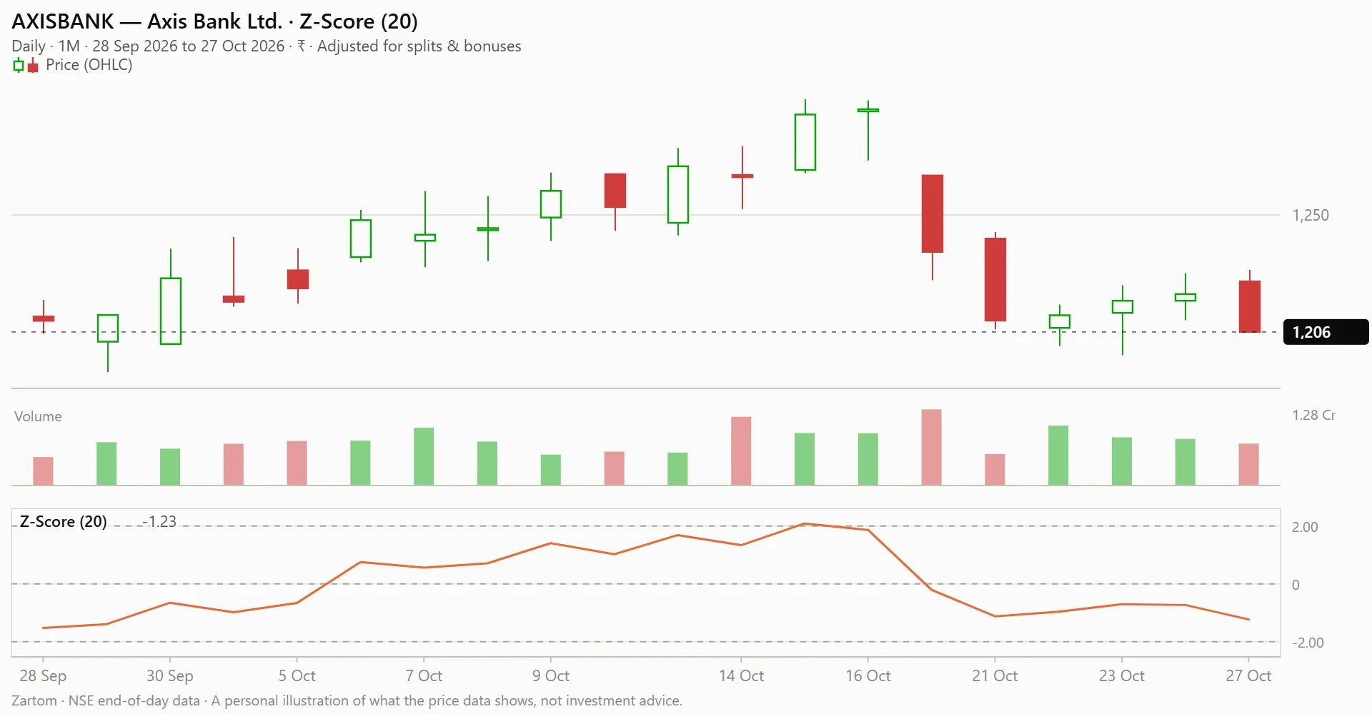
Chart: Z-Score (20)

The Z-Score chart shows the daily price with volume at the base and a 20-period standardised score plotted beneath. The score expresses how many standard deviations the close is above or below its recent average, which turns an absolute price gap into a volatility-adjusted one and makes readings comparable across different market conditions.

Z-Score (20): what it shows

The Z-Score measures how many standard deviations the close is above or below its N-day average, with N set to 20 here. The current reading is -1.23, meaning the close is 1.23 standard deviations below its recent average.

Over the last year the score ranged from -3.71 to 3.1 with a median of 0.3889, so today's value sits at the 18th percentile of that distribution.

The score has moved sharply lower in the short term. It changed by −1.02 over the last five sessions but only −0.07 over the last 20, which indicates that most of the recent decline in the reading happened within the past week.

Of the last 252 readings, 16 (6%) were above 2 and 14 (6%) were below -2, and the latest reading sits between those thresholds.

The line last rose through 2 on 15 October 2026 and last fell through -2 on 24 September 2026. Those crossings mark the moments when the close moved more than two standard deviations from its 20-day average, which is a relatively rare event given that only 12% of the year's readings fell outside that band in either direction.

The calculation behind this indicator, with a worked example from this stock's own prices, is shown below.

Learn: how the Z-Score (20) is calculated

How many standard deviations the close is above or below its N-day average.

Statistical indicators describe how unusual the current price is compared with its own recent history (a z-score, a regression line, a percentile).

Settings for this chart: Period = 20.

The general pattern of this family in Python

import pandas as pd

# a pattern for the statistics family, not the exact formula of Z-Score
z = (close - close.rolling(window).mean()) / close.rolling(window).std()

Every indicator in this family depends on its window length and on how the first values are started, so two charting programs can show slightly different numbers for the same settings. The exact definition used by this app is the one printed in the indicator's description above.

Chart: LinReg (20)

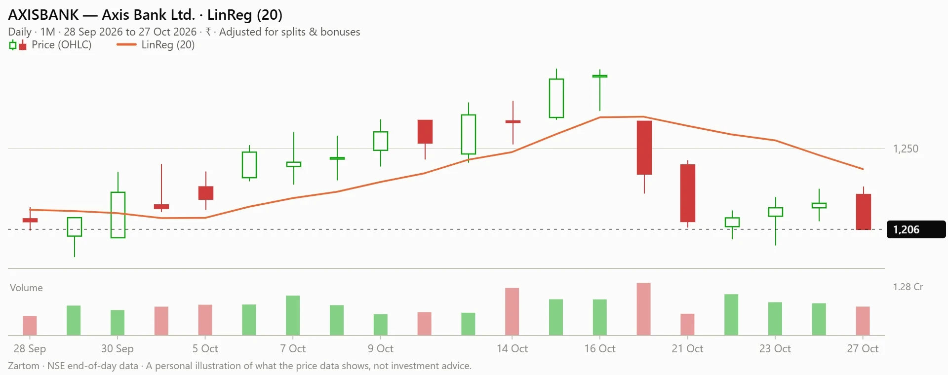
The linear regression chart plots the daily price with volume at the base and the endpoint of a 20-period least-squares line drawn through the closes. Unlike a simple average, which weights every close equally, the regression line fits a straight trend to the recent data and its endpoint reflects both the level and the slope of that fit.

LinReg (20): what it shows

The linear regression line is the end of the least-squares straight line through the last N closes, with N set to 20. The current value is 1,239, and the close of 1,206 is 2.7% below it.

Over the last year the line ranged from 1,155 to 1,410 with a median of 1,266, placing today's value at the 29th percentile of that range.

The line's own direction is a study in contrast. It changed by −28.60 over the last five sessions but rose by +16.90 over the last 20, and it has risen 1.4% over the 20-session window.

That combination describes a line whose underlying slope over the month was upward even as the most recent week pulled the endpoint sharply lower.

The close last crossed below the regression line on 19 October 2026, and it crossed the line 51 times over the last year. A crossing count that high reflects a price that has oscillated around its fitted trend rather than trending cleanly on one side of it for extended periods.

The calculation behind this indicator, with a worked example from this stock's own prices, is shown below.

Learn: how the LinReg (20) is calculated

The end of the least-squares straight line through the last N closes.

Trend indicators smooth or bound the price so its general direction is easier to see. Most are built from a rolling window of recent prices: a plain average, a weighted average, or a band around one.

Settings for this chart: Period = 20.

The general pattern of this family in Python

import pandas as pd

# a pattern for the trend family, not the exact formula of Linear Regression
close.rolling(window).mean()      # a plain rolling average
close.ewm(span=window).mean()     # an exponentially weighted average

Every indicator in this family depends on its window length and on how the first values are started, so two charting programs can show slightly different numbers for the same settings. The exact definition used by this app is the one printed in the indicator's description above.

Corporate actions in the last 12 months

Corporate actions adjust the cash flows attached to a share and can affect how price series are interpreted over time. The record for Axis Bank over the last 12 months contains a single entry: a dividend of ₹1 per share with an ex-date of 10 July 2026. No splits, bonus issues or other capital events appear in the brief for this window.

Last five sessions

The five most recent sessions show how the current close was reached. The sequence opens on 21 October 2026 with a close of 1,210.00 after an open of 1,241.00, then moves through 1,212.00, 1,217.50 and 1,220.00 before the final print of 1,205.70 on 27 October 2026. Volume ranged from 52.8 L to 1.00 Cr across the five days.

The pattern across the five days is a rise from 1,210.00 to 1,220.00 followed by a single session that gave back more than that gain. The 27 October close of 1,205.70 was the lowest of the five, and the session's high of 1,229.20 was also the highest of the week, so the day's range was wide relative to its close.

Learn: the mathematics of returns, volatility and drawdown

The figures quoted throughout this note are not arbitrary; each is the output of a specific calculation applied to the stored price series. Return is the percentage change between two closes, and the multi-period figures in the returns table are built from the same simple formula applied over different lookbacks.

Volatility scales the standard deviation of daily returns to an annual basis, and drawdown tracks the deepest fall from a running peak.

For Axis Bank, the brief records a CAGR of 0.8% and a volatility of 23.3% over the measured windows. Those two numbers sit alongside the return and drawdown figures already discussed, and together they describe a stock whose long-run compounding has been modest while its short-run price swings have been meaningful. The block below sets out the formulas and a worked example using this stock's own prices.

The mathematics behind these measures, with a worked example from this stock's own prices, is shown below.

Learn: the mathematics of returns, volatility and drawdown

Three numbers describe most of what a price history has done: how much it gained, how bumpy the ride was, and how deep the worst fall was. Here is how each is calculated, with this instrument's own figures.

Return, and the yearly growth rate (CAGR)

From 16 Oct 2025 to 27 Oct 2026 (1.03 years) the close went from ₹1,196.30 to ₹1,205.70.

###R = \frac{P_{\text{end}}}{P_{\text{start}}} - 1 = \frac{1205.70}{1196.30} - 1 = 0.8\%###

The compound annual growth rate is the steady yearly rate that gives the same result:

###\text{CAGR} = \left(\frac{P_{\text{end}}}{P_{\text{start}}}\right)^{1/\text{years}} - 1 = 0.8\%###

Daily log returns and volatility

Daily changes are usually measured as logarithmic returns because they add up over time:

###r_t = \ln\frac{C_t}{C_{t-1}}###

The standard deviation of the last 60 daily log returns of this instrument is 1.47%. Scaling it to a year multiplies by the square root of the number of trading days (about 252):

###\sigma_{\text{annual}} = \sigma_{\text{daily}}\sqrt{252} = 1.47\% \times 15.87 = 23.3\%###

Drawdown

###D_t = \frac{C_t}{\max_{s \le t} C_s} - 1###

The deepest value of this in the last year was -17.2%.

In Python (pandas)

import numpy as np
import pandas as pd

def summary(close: pd.Series, trading_days: int = 252) -> dict:
    log_ret = np.log(close / close.shift(1)).dropna()
    years = len(close) / trading_days
    return {
        "return": close.iloc[-1] / close.iloc[0] - 1,
        "cagr": (close.iloc[-1] / close.iloc[0]) ** (1 / years) - 1,
        "volatility": log_ret.std(ddof=1) * np.sqrt(trading_days),
        "max_drawdown": (close / close.cummax() - 1).min(),
    }

Going deeper

• Percentage returns multiply (a 10% gain then a 10% loss leaves 99%), while log returns add; that is why volatility is measured on log returns and why averaging percentage returns overstates growth.
• For small daily changes the two are almost equal: ln(1 + r) ≈ r − r²/2.
• A volatile path grows more slowly than its average return suggests. For a lognormal price the growth rate is about the average return minus half the variance:
• The square-root-of-time rule assumes daily returns are independent and equally volatile. Volatility clusters (calm and stormy periods), so a yearly figure scaled from 60 days is an estimate of the recent regime, not a law.
• Drawdown has memory: a price that fell 50% needs a 100% rise to recover, and the time spent below a previous high matters as much as the depth.

###\text{CAGR} \approx \mu - \frac{\sigma^2}{2}###

With the annualised volatility of 23.3% above, the term ##\sigma^2/2## is 2.7 percentage points a year of "volatility drag" if the average yearly return ##\mu## were measured on log returns.

A further Python version: rolling volatility and drawdown depth

def rolling_risk(close, window=60, trading_days=252):
    log_ret = np.log(close / close.shift(1))
    vol = log_ret.rolling(window).std(ddof=1) * np.sqrt(trading_days)
    drawdown = close / close.cummax() - 1
    underwater = (drawdown < 0).astype(int).groupby((drawdown == 0).cumsum()).cumsum()   # days since the last high
    return pd.DataFrame({"volatility": vol, "drawdown": drawdown, "days_below_high": underwater})

Disclaimer: This article is for general information and education only. It describes what historical prices and technical indicators showed on the date mentioned and does not predict future movements. It is not investment advice, a recommendation, or an offer to buy or sell any security.

Indicators are calculated from past data and can mislead, and all investments carry risk. Please consult a SEBI-registered investment adviser before making any financial decision.